Err... to R! - Building functions

Can we build it? After a couple of attempts, probably, yeah.

January 22, 2018 Simon Wallace

12 minute read

Can we build it? After a couple of attempts, probably, yeah.

This is it. This post will guide you through building a function, from the general form to an example using the topics covered in this series. A rule of thumb I like is if you write the same piece of code three or more times you should put it into a function, because you are using it consistently.

Building a function

A function is just a set of code that we can use repeatedly and returns a predetermined value. When defining a function we have a function name, arguments that the function will take, and the code the function will execute like so:

FUNCTION_NAME <- function(ARGUMENTS){
  CODE
}

A function evaluates within its own environment, so unless we specify we want the variables within a function to be available outside of it they will be deleted upon completion. The most common way of doing this is through returning a value at the end of the function:

FUNCTION_NAME <- function(ARGUMENTS){
  CODE
  return(VALUE)
}

Whilst we can place a return anywhere in a function, but nothing will be evaluated after the return as the function stops once it has returned a value.

One of the first pieces of code we wrote in this series was:

value <- 2
2*value

## [1] 4

Let us now turn it into a function:

my_first_func <- function(x){
  y <- 2*x
  return(y)
}

We run, or call, the function like so:

my_first_func(value)

## [1] 4

If you remember ls() will return all the variables within our environment, and as the variable y only exists locally within in my_first_func it does not exist globally.

ls()

## [1] "my_first_func" "value"

'y'%in%ls()

## [1] FALSE

As you can see defining a function is similar to defining a variable, albeit with a slightly higher level of complexity. As we did previously we can see the class of the variable my_first_func:

class(my_first_func)

## [1] "function"

Argument values

Within our function definition we can specify default values that the function will use unless specified otherwise.

func <- function(x=1,y=2){
  val <- x*y
  return(val)
}
func()

## [1] 2

If we want to change the value of y we can do so by assigning it a value within the function call like so:

func(y=3)

## [1] 3

func(y <- 4)

## [1] 8

You can use either assignment within a function call, however in a definition you must use =

func <- function(x=1,y<-2){
  val <- x*y
  return(val)
}

## Error: <text>:1:23: unexpected assignment
## 1: func <- function(x=1,y<-
##                           ^

Order in evaluation

As we mentioned in the post where we introduced the pipe, it pipes a value into the first available argument within a function. By available we meant unspecified within the function call, as if we do not specify the variable then even if the first variable has a default value it will be overridden.

pipeFunc <- function(w=4,x,y,z){
  val <- w*x+y*z
  print(paste('w,x,y,z=c(',w,',',x,',',y,',',z,')',sep=''))
  return(val)
}
5 %>%
pipeFunc(w=2,x=3,z=5)

## [1] "w,x,y,z=c(2,3,5,5)"

## [1] 31

5 %>%
pipeFunc(x=3,z=5)

## Error in pipeFunc(., x = 3, z = 5): argument "y" is missing, with no default

The last evaluation failed because 5 was assigned to the variable w and because y has no default value and was not specified the function fails.

This is the same in standard evaluations and is why we should place arguments with default values at the end within the function definition:

pipeFunc(1,2,3)

## Error in pipeFunc(1, 2, 3): argument "z" is missing, with no default

pipeFixed <- function(x,y,z,w=4){
  val <- w*x+y*z
  print(paste('w,x,y,z=c(',w,',',x,',',y,',',z,')',sep=''))
  return(val)
}
pipeFixed(1,2,3)

## [1] "w,x,y,z=c(4,1,2,3)"

## [1] 10

As such when we are specifying the arguments in a function call we should exercise caution to ensure the right value is going to the right argument, if in doubt specify the argument you want the value to be assigned to in the call.

Global parameters within functions

As we discussed the the loops post, variables are stored to either a global or local environment depending on where they are declared. Parameters created in a function like val are within the function’s local environment and are not available in the global environment. Although the parameters within a function are not automatically available in the global environemnt, we can access parameters from the global environment within the function. This can cause problems upon evaluation if we repeat a variable name and as such we should try to avoid variable name duplication within our function.

For example we specified value at the top of this post:

func <- function(y){
  return(y*value)
}
func(3)

## [1] 6

The function evaluated because value exists within the global environment. However if we specify it as an argument within the function definition the global variable is not used:

func <- function(y,value){
  return(y*value)
}
func(3)

## Error in func(3): argument "value" is missing, with no default

We need to specify both arguments for the function to evaluate.

func(value=2,y=2)

## [1] 4

If for some reason we need to duplicate variable names then we should include them in the argument definition of a function for safety, otherwise this is an area where we can create code that does not function as expected.

Building functions

Functions don’t have to be 200 line behemoths, they can be as we illustrated short pieces of code we want easy access to. However, if we are building a behemoth function we need to be careful during creation otherwise the debugging will be tortuous.

From experience - aka blood, sweat and tears - creating the function should be the last thing we do to a piece of code. This is because we have a greater level of control and detail when building if we can evaluate each line and check it is performing as expected. So, when building a function I would recommend building it as lines of code then encapsulating the code within a function when we know it works. In this case we have to be careful regarding the global vs. local evaluation and it is recommended to clear your workspace before testing the function.

We are now going to build a function that will create a bar chart for a column specified within mtcars. Whilst this may not seem too difficult, there are checks that we need to put in place on the data and will use all of the topics covered until now.

mtBarChart

When building a function I like to think of what the potential inputs are going to be and what the output we desire is. In this case our output is a graph and our inputs is going to be a string representing a column name that specifies the xaxis within the barchart.

Let us start simple, and build this count bar chart which requires one input that we can use as an x axis grouping variable.

target <- ggplot(mtcars_tibble)+
  geom_bar(aes(x=as.factor(cyl)))
target

Now we know what the target outcome of our function is, let us start building the code.

One of our inputs is going to be a string representing a column name, whilst in ggplot2 we can specify a string as a plotting aesthetic it will plot against that string rather than against the variable.

x_column <- 'cyl'
ggplot(mtcars_tibble)+
  geom_bar(aes(x=x_column))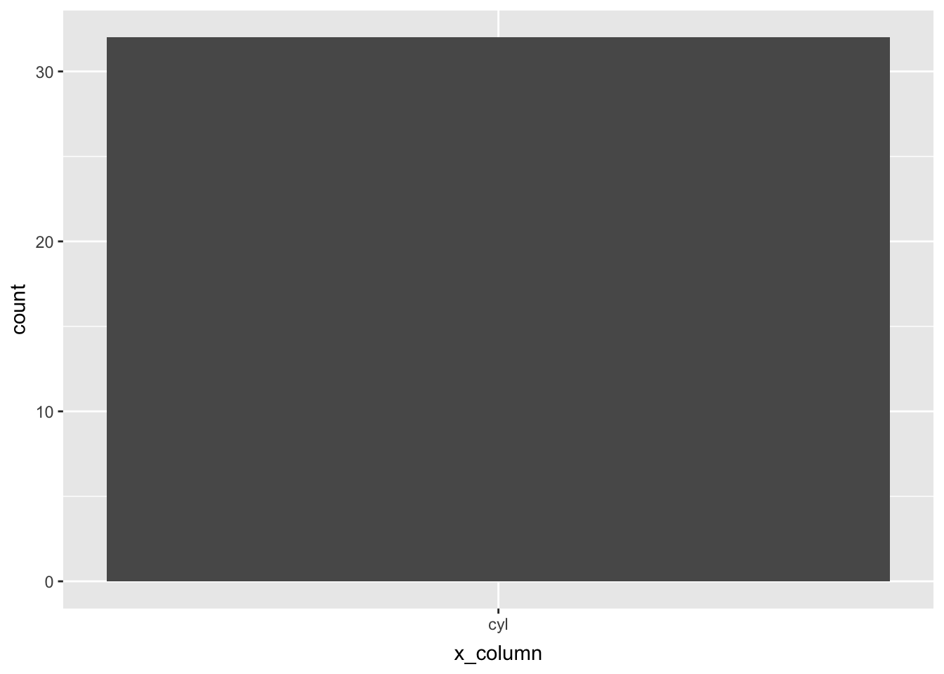

Good news though, within ggplot2 geoms there is an aesthetic function that can take strings aes_string() that solves this problem; so rather than plotting against the string it will look for the column within our specified dataset.

x_column <- 'cyl'
ggplot(mtcars_tibble)+
  geom_bar(aes_string(x=x_column))

We are almost there. However we run into the problem that the x axis is being created as a continuous variable, we should make it so any column specified as the x_column is automatically converted to a factor.

In the pipe below we have created a column called “x_column” which is a factor version of the column ‘cyl’ within the data. Remember that within a pipe . specifies the data being piped - in this case mtcars_tibble and we can select a column within a data set using [[]].

x_column <- 'cyl'
plottingData <- mtcars_tibble %>%
  mutate(x_column=as.factor(.[[x_column]]))

However the problem is that when we create the new column it is created as ‘x_column’ not replacing ‘cyl’ because dplyr doesn’t require strings as variable names. Within the package magrittr there is a function called set_colnames() that will fix this problem if we only select the columns that we need. This may not be the only solution to the problem, but if we come across a better way in the future we can iterate our function accordingly.

x_column <- 'cyl'
plottingData <- mtcars_tibble %>%
  mutate(x_column=as.factor(.[[x_column]])) %>%
  select(x_column)%>%
  set_colnames(x_column)

ggplot(plottingData)+
  geom_bar(aes_string(x=x_column))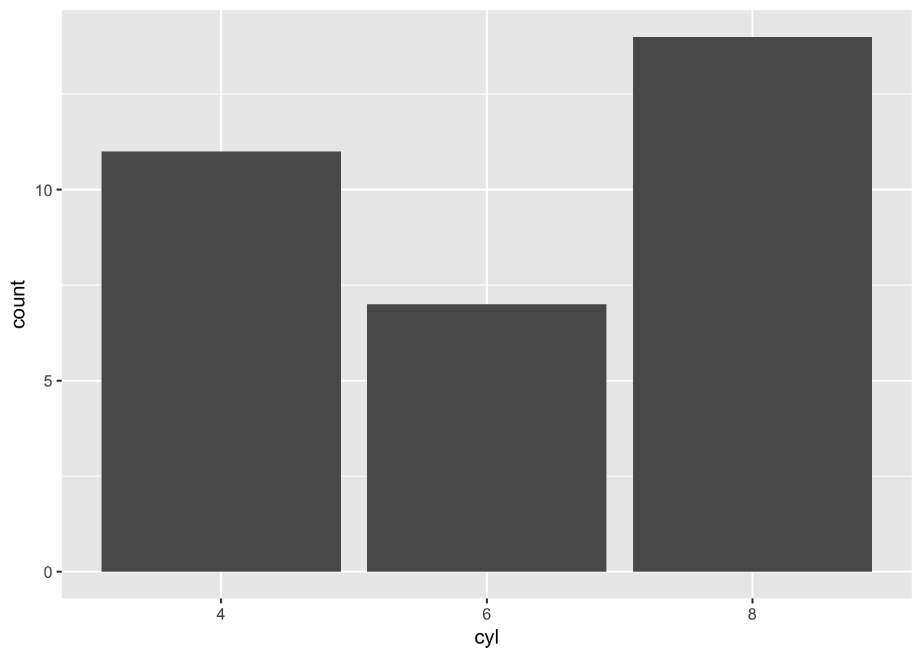

This illustrates a point we discussed in the data variables and manipulation post; dplyr uses “bare” names and so creates “x_column” as a variable, whereas magrittr will use the value assigned to the variable x_column. This is where using multiple packages can start to get a bit tricky but as long as you are aware of the differences they become easy to spot like we did above.

Let us now wrap this in a function:

mtBarChart <- function(x_column){
  plottingData <- mtcars_tibble %>%
  mutate(x_column=as.factor(.[[x_column]])) %>%
  select(x_column)%>%
  set_colnames(x_column)

 plot <- ggplot(plottingData)+
  geom_bar(aes_string(x=x_column))
 return(plot)
}
mtBarChart('cyl')

It works as expected! Now let’s try and break it.

Debugging and testing

Functions have to be able to return a value consistently, so if there is a value that breaks the function or stops it performing as intended we need to either fix the problem or stop the evaluation in a controlled way.

For example the fact that cyl was being treated as a numeric value rather than a factor was stopping our function behaving in an intended way and we fixed it. This fix will work for all variables apart from one type - floats.

mtBarChart('disp')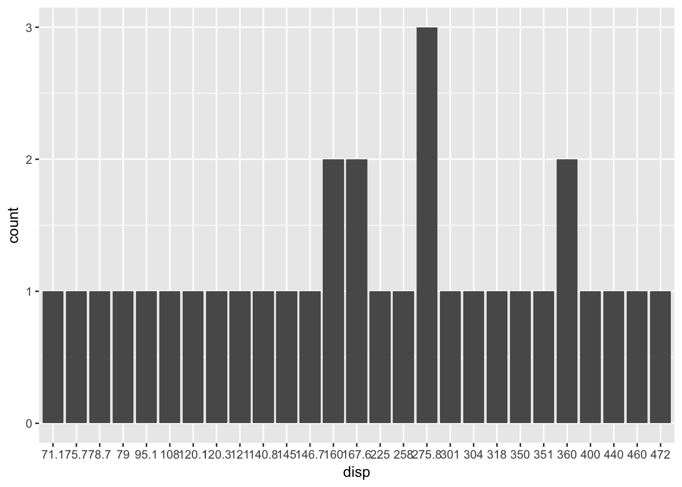

We could either create a new variable which groups together our values or stop the function because it isn’t a variable class we intended this plot to be used for. We will go for the second option, which requires us to use a conditional.

A way in which we can check if a vector is a float or an integer is to see if the number of unique elements is the same after rounding, like so:

length(unique(round(column)))==length(unique(column))

So let us place this as a conditional in our function and cause an error if we pass a float into this function.

mtBarChart <- function(x_column){
  if(length(unique(round(mtcars_tibble[[x_column]])))==length(unique(mtcars_tibble[[x_column]]))){
      plottingData <- mtcars_tibble %>%
        mutate(x_column=as.factor(.[[x_column]])) %>%
        select(x_column)%>%
        set_colnames(x_column)
      
      plot <- ggplot(plottingData)+
        geom_bar(aes_string(x=x_column))
      return(plot)
  }else{
    stop('Bar plots should not be used with a float x axis')
  }
}
mtBarChart('cyl')

mtBarChart('disp')

## Error in mtBarChart("disp"): Bar plots should not be used with a float x axis

It works, but that error message doesn’t help anyone. Perhaps we could create a message that identifies columns that could be used in our function. We could do this by looping through the columns within mtcars_tibble looking for either character variables or integers.

We will create a loop where we go through each column name within mtcars_tibble and see whether it is an integer, character or factor and therefore can be used as an x axis within a bar chart.

mtBarChart <- function(x_column){
  if(length(unique(round(mtcars_tibble[[x_column]])))==length(unique(mtcars_tibble[[x_column]]))){
      plottingData <- mtcars_tibble %>%
        mutate(x_column=as.factor(.[[x_column]])) %>%
        select(x_column)%>%
        set_colnames(x_column)
      
      plot <- ggplot(plottingData)+
        geom_bar(aes_string(x=x_column))
      return(plot)
  }else{
    potential <- character()
    for(col in colnames(mtcars_tibble)){
      if(is.character(mtcars_tibble[[col]])|is.factor(mtcars_tibble[[col]])|length(unique(round(mtcars_tibble[[col]])))==length(unique(mtcars_tibble[[col]]))){
        potential[length(potential)+1] <- col
      }
    }
    stop('Bar plots should not be used with a float x axis. You could use the following columns: ',paste(potential,collapse=', '))
  }
}
mtBarChart('disp')

## Error in mtBarChart("disp"): Bar plots should not be used with a float x axis. You could use the following columns: cyl, hp, vs, am, gear, carb

There it is, a working and fairly robust function. The only problem is that functions should be designed to work for any dataset, not just one as in our case. Let’s test that now:

barChart <- function(data,x_column){
  if(length(unique(round(data[[x_column]])))==length(unique(data[[x_column]]))){
    plottingData <- data %>%
      mutate(x_column=as.factor(.[[x_column]])) %>%
      select(x_column)%>%
      set_colnames(x_column)
    
    plot <- ggplot(plottingData)+
      geom_bar(aes_string(x=x_column))
    return(plot)
  }else{
    potential <- character()
    for(col in colnames(data)){
      if(is.character(data[[col]])|is.factor(data[[col]])|length(unique(round(data[[col]])))==length(unique(data[[col]]))){
        potential[length(potential)+1] <- col
      }
    }
    stop('Bar plots should not be used with a float x axis. You could use the following columns: ',paste(potential,collapse=', '))
  }
}
barChart(mtcars,'cyl')

Let’s try this with another dataset which you should be familiar with from the exercises:

barChart(iris,'Species')

## Error in Math.factor(structure(c(1L, 1L, 1L, 1L, 1L, 1L, 1L, 1L, 1L, 1L, : 'round' not meaningful for factors

This error is because we are trying to round a factor, which can’t be done. We need to change our conditionals, so they are nested to check for errors before evaluation.

if(!CHARACTER|!FACTOR){
  if(FLOAT){
    ERROR
  }
}

barChart <- function(data,x_column){
  if(!(is.character(data[[x_column]])|is.factor(data[[x_column]]))){
      if(!(length(unique(round(data[[x_column]])))==length(unique(data[[x_column]])))){
        potential <- character()
          for(col in colnames(data)){
            if(is.character(data[[col]])|is.factor(data[[col]])){
              potential[length(potential)+1] <- col
            }else if(length(unique(round(data[[col]])))==length(unique(data[[col]]))){
              potential[length(potential)+1] <- col
            }
        stop('Bar plots should not be used with a float x axis. You could use the following columns: ',paste(potential,collapse=', '))
      }
    }
  }
  plottingData <- data %>%
      mutate(x_column=as.factor(.[[x_column]])) %>%
      select(x_column)%>%
      set_colnames(x_column)
    
    plot <- ggplot(plottingData)+
      geom_bar(aes_string(x=x_column))
    return(plot)
}
barChart(iris,'Species')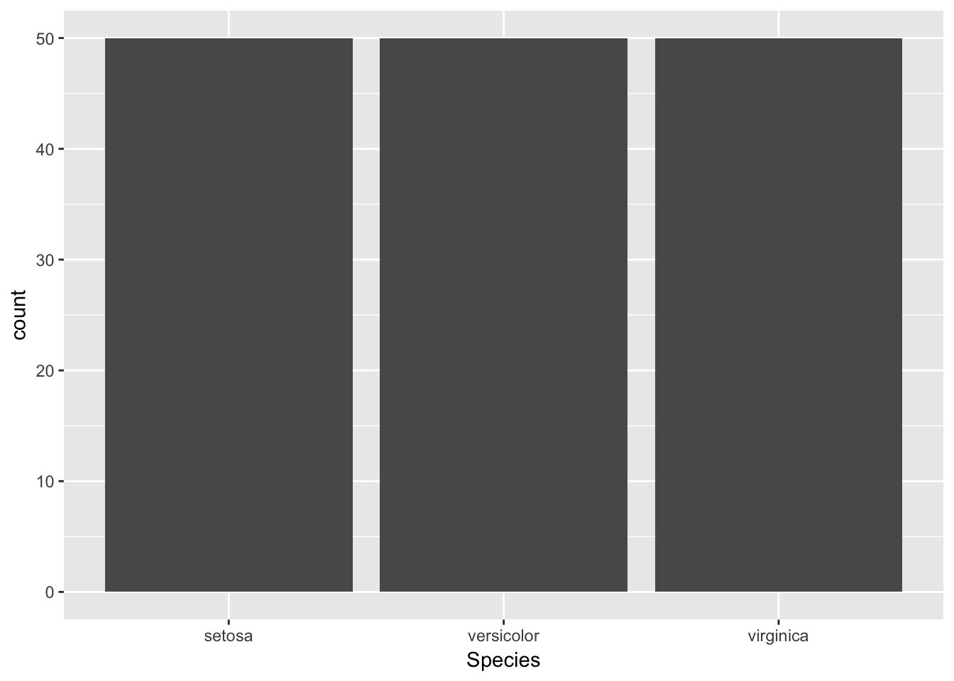

barChart(mtcars,'cyl')

Finally it is best practice to comment a function so that it is understood what is happening at each stage. Both for yourself upon future investigation and for anyone else who might read your function.

barChart <- function(data,x_column){
  # This function creates a count bar chart with a factor, character, or integer x axis
  if(!(is.character(data[[x_column]])|is.factor(data[[x_column]]))){
    # Not a character or factor 
      if(!(length(unique(round(data[[x_column]])))==length(unique(data[[x_column]])))){
        # Column is a float
        potential <- character()
        # Identifying valid columns
        for(col in colnames(data)){
          if(is.character(data[[col]])|is.factor(data[[col]])){
            potential[length(potential)+1] <- col
          }else if(length(unique(round(data[[col]])))==length(unique(data[[col]]))){
            potential[length(potential)+1] <- col
          }
        # Terminating function with suggested columns
        stop('Bar plots should not be used with a float x axis. You could use the following columns: ',paste(potential,collapse=', '))
      }
    }
  }
  # Creating plotting data
  plottingData <- data %>%
    # Converting to factor to ensure x axis is categorical in case of integer
      mutate(x_column=as.factor(.[[x_column]])) %>%
    # Selecting only the x_column as dplyr has created data[['x_column']]
      select(x_column)%>%
    # Renaming data[['x_column']] to the string specified in the arguments
      set_colnames(x_column)
    # Creating plot
    plot <- ggplot(plottingData)+
      geom_bar(aes_string(x=x_column))
    # Returning plot
    return(plot)
}

Code, Problems, and Solutions

The final set of coding problems are here. This time they are slightly different as we will be iterating the barChart() function we have created. Once you have finished these however you should look at discovering your own problem you want to build a function for - because that is what coding is all about.

About “Err… to R!” posts

The general desire to learn a programming language is increasing. Whilst R has a fairly steep learning curve in comparison to other languages, it was designed to analyse data. Once you take into account CRAN, R is one of the most powerful analytics tools available. The goal of this course is to get you comfortable using R, and the way in which it shall be presented is such that you can hopefully learn another language - if wanted/needed - quickly as the way in which the material is presented is designed to help you understand how to learn a programming language; not just how to learn R.

Statistician Six

Blog

Categories

About

Recent Posts